2  Chapter 02: Probability

2.1 Problem 2.1

When rolling two dice, what is the probability that one die is twice the other?

Besides the classical way of enumerating all events outcomes, we can also tackle this problem in the following way:

let’s consider two dice - one black and one white. The event that one die shows twice what the other die shows can be thought of as the union of two events: either the black die shows twice what the white die shows (Event A), or the white die shows twice what the black die shows (Event B). These two events are mutually exclusive, so the probability of either event happening is the sum of the probabilities of each event happening.

Now, let’s suppose we roll the black die first and then the white die. If the black die shows an odd number, then we know that Event A cannot happen. However, if the black die shows an even number, there is exactly one number on the white die that will result in Event A happening. Since there are n possible numbers on a die (assuming n is even), the probability of Event A happening is \frac{1}{2} \cdot \frac{1}{n}.

By symmetry, the probability of Event B happening is also \frac{1}{2} \cdot \frac{1}{n}. Therefore, the probability of either Event A or Event B happening is P(A \cup B) = 2 \cdot \frac{1}{2} \cdot \frac{1}{n}.

comming back to our particular case, it means:

P(E) = 2 \cdot \frac{1}{2} \cdot \frac{1}{6} = \frac{1}{6}

we can simulate this experiment in R as follow:

event <- replicate(100000, {
    die_1 <- sample(x = 1:6, size = 1, replace = TRUE)
    die_2 <- sample(x = 1:6, size = 1, replace = TRUE)
    (die_1 == 2 * die_2) | (die_2 == 2 * die_1)
})
mean(event)

[1] 0.16729

2.2 Problem 2.2

Consider an experiment where you roll two dice, and subtract the smaller value from the larger value (getting 0 in case of a tie).

1. What is the probability of getting 0?
2. What is the probability of getting 4?

2.2.1 Part (a)

The probability of getting 0 is the probability of getting a tie. This is the probability of getting the same number on both dice.

E = \{(1,1), (2,2), (3,3), (4,4), (5,5), (6,6) \}

and we have 6 \cdot 6 = 36 possible outcomes. So:

P(E) = \frac{6}{36} = \frac{1}{6}

we can simulate this experiment in R as follow:

event <- replicate(100000, {
    die_1 <- sample(x = 1:6, size = 1, replace = TRUE)
    die_2 <- sample(x = 1:6, size = 1, replace = TRUE)
    die_1 == die_2
})
mean(event)

[1] 0.16885

2.2.2 Part (b)

The probability of getting 4 is the probability of getting a difference of 4.

E = \{(1,5), (5,1), (2,6), (6,2) \}

and we have 6 \cdot 6 = 36 possible outcomes. So:

P(E) = \frac{4}{36} = \frac{1}{9}

we can simulate this experiment in R as follow:

event <- replicate(100000, {
    die_1 <- sample(x = 1:6, size = 1, replace = TRUE)
    die_2 <- sample(x = 1:6, size = 1, replace = TRUE)
    abs(die_1 - die_2) == 4
})
mean(event)

[1] 0.11138

2.3 Problem 2.3

A hat contains slips of paper numbered 1 through 6. You draw two slips of paper at random from the hat, without replacing the first slip into the hat.

1. Write out the sample space S for this experiment.
2. Write out the event E “the sum of the numbers on the slips of paper is 4”.
3. Find P(E).
4. Let F be the event “the larger number minus the smaller number is 0”. What is P(F)?

2.3.1 Part (a)

We can write the sample space as:

S = \{(1,2), (1,3), \cdots , (6,5) \}

2.3.2 Part (b)

We can write the event as:

E = \{(1,3), (3,1) \}

2.3.3 Part (c)

We have 6 \cdot 5 = 30 possible outcomes. So:

P(E) = \frac{2}{30} = \frac{1}{15}

we can simulate it in R as follows:

event <- replicate(100000, {
    hat <- sample(x = 1:6, size = 2, replace = FALSE)
    sum(hat) == 4
})
mean(event)

[1] 0.06602

2.3.4 Part (d)

Since we cannot draw the same number twice:

F = \emptyset

P(F) = 0

2.4 Problem 2.4

Suppose there are two boxes and each contain slips of papers numbered 1-8. You draw one number at random from each box.

1. Estimate the probability that the sum of the numbers is 8.
2. Estimate the probability that at least one of the numbers is a 2.

2.4.1 Part (a)

There are 8 \cdot 8 = 64 possible outcomes. The number of outcomes where the sum is 8 is:

E = \{(1,7), (2,6), \cdots, (7,1) \} and the probability is:

P(E) = \frac{7}{64}

We can simulate this experiment in R as follows:

event <- replicate(100000, {
    box_1 <- sample(x = 1:8, size = 1, replace = TRUE)
    box_2 <- sample(x = 1:8, size = 1, replace = TRUE)
    sum(box_1 + box_2) == 8
})
mean(event)

[1] 0.10945

2.4.2 Part (b)

Similarly, the number of outcomes where at least one of the numbers is 2 is:

E = \{(1,2), (2,1), (2,2), (2,3), \cdots, (8,2) \}

and the probability is:

P(E) = \frac{15}{64}

We can simulate this experiment in R as follows:

event <- replicate(100000, {
    box_1 <- sample(x = 1:8, size = 1, replace = TRUE)
    box_2 <- sample(x = 1:8, size = 1, replace = TRUE)
    box_1 == 2 | box_2 == 2
})
mean(event)

[1] 0.23232

2.5 Problem 2.5

Suppose the proportion of M&M’s by color is:

Color	Proportion
Yellow	0.14
Red	0.13
Orange	0.20
Brown	0.12
Green	0.20
Blue	0.21

1. What is the probability that a randomly selected M&M is not green?
2. What is the probability that a randomly selected M&M is red, orange, or yellow?
3. Estimate the probability that a random selection of four M&M’s will contain a blue one.
4. Estimate the probability that a random selection of six M&M’s will contain all six colors.

2.5.1 Part (a)

Using the law of complement, we have:

P(\neg \text{G}) = 1 - P(\text{G}) = 0.80

2.5.2 Part (b)

We can use the law of addition to find the probability of getting red, orange, or yellow:

P(\text{R} \cup \text{O} \cup \text{Y}) = P(\text{R}) + P(\text{O}) + P(\text{Y})

P(\text{R} \cup \text{O} \cup \text{Y}) = 0.13 + 0.20 + 0.14

P(\text{R} \cup \text{O} \cup \text{Y}) = 0.47

2.5.3 Part (c)

By the law of complement the probability of not getting a blue is 1 - 0.21 = 0.79 and the probability of not getting a blue in four selections is (0.79)^4 = 0.39. Then the probability of getting at least one blue in four selections is:

• E: at least one blue in four selections

P(E) = 1 - P(\neg E) = 1 - 0.39 = 0.61

We can simulate this experiment in R as follows:

event <- replicate(100000, {
    mms <- sample(x = c("yellow", "red", "orange", "brown", "green", "blue"),
     size = 4, p = c(0.14, 0.13, 0.20, 0.12, 0.20, 0.21), replace = TRUE)
    "blue" %in% mms
})
mean(event)

[1] 0.61046

2.5.4 Part (d)

The probability of selecting six M&M’s that contain all six colors is (consdiering ordering):

• E: All colors with an specific order P(E) = 0.14 \cdot 0.13 \cdots 0.21

we need to calculate the total number of ways we can select six M&M’s from a total of 6 colors, with a sample size of 6. That is 6!. Then the probability is:

• F: All six colors no matter order

P(F) = 6! \cdot P(E) = 0.0132

We can simulate this experiment in R as follows:

event <- replicate(100000, {
    mms <- sample(x = c("yellow", "red", "orange", "brown", "green", "blue"),
     size = 6, p = c(0.14, 0.13, 0.20, 0.12, 0.20, 0.21), replace = TRUE)
    length(unique(mms)) == 6
})
mean(event)

[1] 0.01337

2.6 Problem 2.6

With the distribution from Problem 2.5, suppose you buy a bag of M&M’s with 30 pieces in it. Estimate the probability of obtaining at least 9 Blue M&M’s and at least 6 Orange M&M’s in the bag.

Warning

Since I’m not quite sure on how to calculate this without the binomial distribution, lets go directly with the R simulation

event <- replicate(100000, {
    mms <- sample(x = c("yellow", "red", "orange", "brown", "green", "blue"),
     size = 30, p = c(0.14, 0.13, 0.20, 0.12, 0.20, 0.21), replace = TRUE)
    sum(mms == "blue") >= 9 & sum(mms == "orange") >= 6
})
mean(event)

[1] 0.06586

2.7 Problem 2.7

Blood types O, A, B, and AB have the following distribution in the United States:

Type	A	AB	B	O
Probability	0.40	0.04	0.11	0.45

What is the probability that two randomly selected people have the same blood type?

Since getting the same blood type is an independent event, we can calculate the probability of getting the same blood type by multiplying the probability of getting each blood type. That is:

• E: Two randomly selected people have the same blood type

P(E) = 0.40^2 + \cdots + 0.45^2 = 0.3762

We can simulate this experiment in R as follows:

event <- replicate(100000, {
    person_1 <- sample(x = c("A", "AB", "B", "O"),
     size = 1, p = c(0.40, 0.04, 0.11, 0.45), replace = TRUE)
    person_2 <- sample(x = c("A", "AB", "B", "O"),
     size = 1, p = c(0.40, 0.04, 0.11, 0.45), replace = TRUE)

    person_1 == person_2
})
mean(event)

[1] 0.37671

2.8 Problem 2.8

Use simulation to estimate the probability that a 10 is obtained when two dice are rolled.

Besides the simulation, we can also calculate the probability of getting a 10. The event space is: E = \{(6,4), (5,5), (4,6)\}

And the possible outcomes are 6 \cdot 6 = 36. Then the probability of getting a 10 is:

P(\text{10}) = \frac{3}{36} = 0.0833

We can simulate this in R as follow:

event <- replicate(100000, {
    dice_1 <- sample(x = 1:6, size = 1, replace = TRUE)
    dice_2 <- sample(x = 1:6, size = 1, replace = TRUE)
    dice_1 + dice_2 == 10
})
mean(event)

[1] 0.08238

2.9 Problem 2.9

Estimate the probability that exactly 3 heads are obtained when 7 coins are tossed.

Since it’s a bit long to calculate this one by counting, lets cite and use the definition of the binomial probability

Tip

Events where there are only two possible outcomes that we can classify as success or failure, and where the probability of success is known to us as p are called binomial events. When we repeat such events several times, the probability to find r successes in n such repetitions can be calculated by using the expression:

P(r) = \binom{n}{r} p^r (1-p)^{n-r}

where \binom{n}{r} is the binomial coefficient, which is the number of ways of selecting r objects from a set of n objects, where the order of selection does not matter.

Knowing that, we can calculate the probability of getting exactly 3 heads in 7 tosses:

• E: Exactly 3 heads P(E) = \binom{7}{3} (0.5)^3 (0.5)^{7-3} = 0.273

We can simulate this in R as follow:

event <- replicate(100000, {
    tosses <- sample(x = c("H", "T"), size = 7, replace = TRUE)
    sum(tosses == "H") == 3
})
mean(event)

[1] 0.27075

We can extend this question by asking what is the probability that at least 3 heads are obtained when 7 coins are tossed. To solve this problem we need to find the probabilities that r could be 3,4,5,6,7 to satisfy the condition “at least”.

• F: At least 3 heads

P(F) = \sum_{r=3}^{7} \binom{7}{r} (0.5)^r (0.5)^{7-r}

r	P(F)
for r = 3	\binom{7}{3} (0.5)^3 (0.5)^{4} = 0.2734375
for r = 4	\binom{7}{4} (0.5)^4 (0.5)^{3} = 0.2734375
for r = 5	\binom{7}{5} (0.5)^5 (0.5)^{2} = 0.1640625
for r = 6	\binom{7}{6} (0.5)^6 (0.5)^{1} = 0.0546875
for r = 7	\binom{7}{7} (0.5)^7 (0.5)^{0} = 0.0078125

P(F) = 0.273 + \cdots + 0.007 = 0.773

We could also have calculated this by using the complement of the probability of getting at most 2 heads.

• G: At most 2 heads P(F) = 1 - P(G)

P(F) = 1 - \sum_{r=0}^{2} \binom{7}{r} (0.5)^r (0.5)^{7-r}

r	P(\text{at most 2 heads})
for r = 0	\binom{7}{0} (0.5)^0 (0.5)^{7} = 0.0078125
for r = 1	\binom{7}{1} (0.5)^1 (0.5)^{6} = 0.0546875
for r = 2	\binom{7}{2} (0.5)^2 (0.5)^{5} = 0.1640625

P(F) = 1 - 0.225 = 0.773

We can simulate this in R as follow:

event <- replicate(100000, {
    tosses <- sample(x = c("H", "T"), size = 7, replace = TRUE)
    sum(tosses == "H") >= 3
})
mean(event)

[1] 0.77311

2.10 Problem 2.10

Estimate the probability that the sum of five dice is between 15 and 20, inclusive.

We need to count the number of ways that we can roll five dice and get a sum between 15 and 20, and divide that by the total number of possible outcomes when rolling five dice. Since it is a bit long to count all possible combinations of (a,b,c,d,e) where a+b+c+d+e \in [15,20] We are going directly with the simulation.

event <- replicate(100000, {
    dice <- sample(x = 1:6, size = 5, replace = TRUE)
    sum(dice) >= 15 & sum(dice) <= 20
})
mean(event)

[1] 0.55585

2.11 Problem 2.11

Suppose a die is tossed repeatedly, and the cumulative sum of all tosses seen is maintained. Estimate the probability that the cumulative sum ever is exactly 20. (Hint: the function cumsum computes the cumulative sums of a vector.)

Again, we are going directly wit the simulation due the overwhelming amount of combinations. We know that 20 is the maximum number of tosses that could have a cumulative sum of 20. So doing a sample of 20 rolls will be enough to get a good estimate.

event <- replicate(100000, {
    tosses <- sample(x = 1:6, size = 20, replace = TRUE)
    cumulative_sum <- cumsum(tosses)
    any(cumulative_sum == 20)
})
mean(event)

[1] 0.28733

2.12 Problem 2.12

(Rolling two dice)

1. Simulate rolling two dice and adding their values. Perform 10,000 simulations and make a bar chart showing how many of each outcome occurred.

2. You can buy trick dice, which look (sort of) like normal dice. One die has numbers 5, 5, 5, 5, 5, 5. The other has numbers 2, 2, 2, 6, 6, 6. Simulate rolling the two trick dice and adding their values. Perform 10,000 simulations and make a bar chart showing how many of each outcome occurred.

3. Sicherman dice also look like normal dice, but have unusual numbers. One die has numbers 1, 2, 2, 3, 3, 4. The other has numbers 1, 3, 4, 5, 6, 8. Simulate rolling the two Sicherman dice and adding their values. Perform 10,000 simulations and make a bar chart showing how many of each outcome occurred. How does your answer compare to part (a)?

2.12.1 Part (a)

library(ggplot2)

outcomes <- replicate(10000, {
    dice_1 <- sample(x = 1:6, size = 1, replace = TRUE)
    dice_2 <- sample(x = 1:6, size = 1, replace = TRUE)
    dice_1 + dice_2
})
df <- data.frame(outcomes)
ggplot(data = df, mapping = aes(outcomes), fill = "transparent") +
geom_histogram(bins = 11, fill = "transparent", color = "black")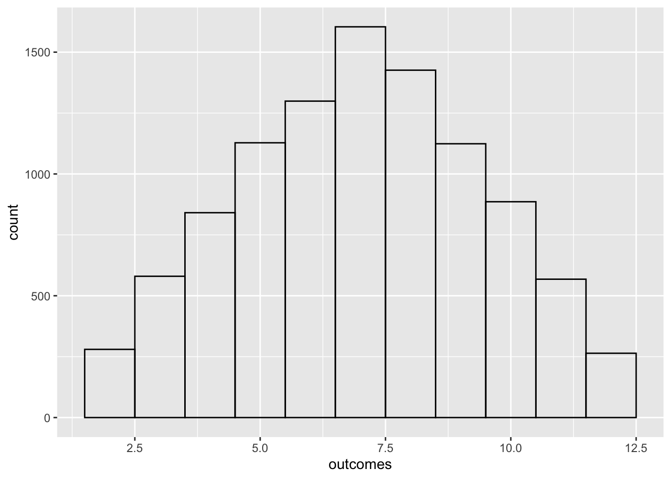

2.12.2 Part (b)

library(ggplot2)

outcomes <- replicate(10000, {
    dice_1 <- sample(x = c(5, 5, 5, 5, 5, 5), size = 1, replace = TRUE)
    dice_2 <- sample(x = c(2, 2, 2, 6, 6, 6), size = 1, replace = TRUE)
    dice_1 + dice_2
})
df <- data.frame(outcomes)
ggplot(data = df, mapping = aes(outcomes), fill = "transparent") +
geom_histogram(bins = 11, fill = "transparent", color = "black")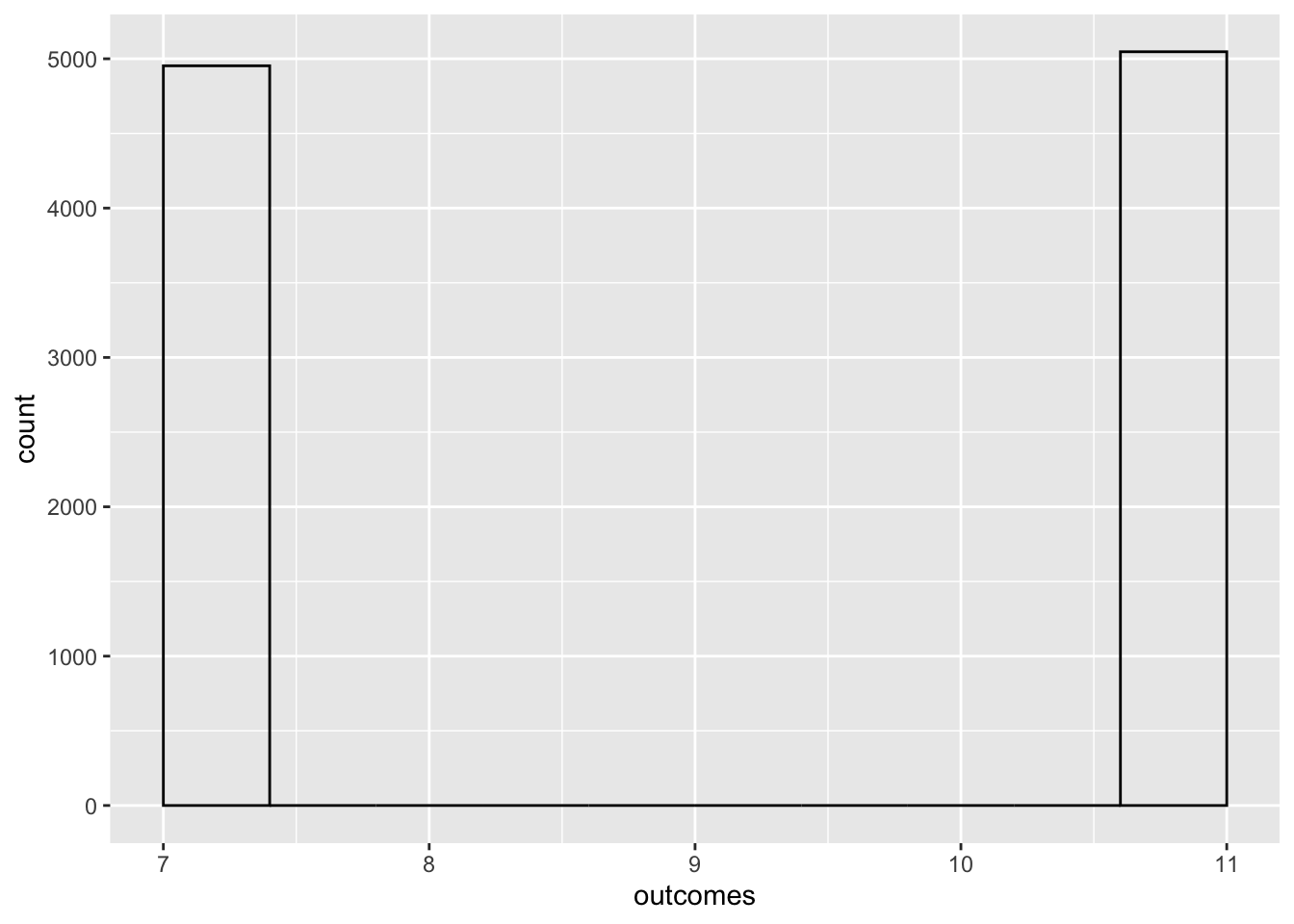

2.12.3 Part (c)

library(ggplot2)

outcomes <- replicate(10000, {
    dice_1 <- sample(x = c(1, 2, 2, 3, 3, 4), size = 1, replace = TRUE)
    dice_2 <- sample(x = c(1, 3, 4, 5, 6, 8), size = 1, replace = TRUE)
    dice_1 + dice_2
})
df <- data.frame(outcomes)
ggplot(data = df, mapping = aes(outcomes), fill = "transparent") +
geom_histogram(bins = 11, fill = "transparent", color = "black")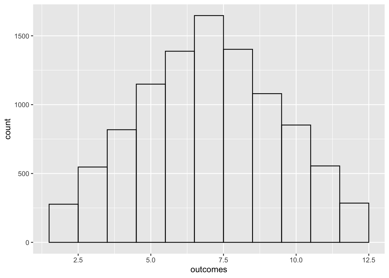

They have the same distribution.

2.13 Problem 2.13

In a room of 200 people (including you), estimate the probability that at least one other person will be born on the same day as you.

we can use the complement rule and calculate the probability that none of the other 199 people share the same birthday as me. Assuming that birthdays are uniformly distributed across all 365 days of the year (ignoring leap years), the probability that any given person in the room was not born on the same day as me is:

• E: No one else has the same birthday as you

P(E) = \left(\frac{1}{365}\right)^{199} = 0.58

And the probability that at least one other person has the same birthday as you is:

• F: At least one other person has the same birthday as you

P(F) = 1 - P(E) = 0.42

we can simulate this in R as follow:

event <- replicate(100000, {
    my_birthday <- sample(x = 1:365, size = 1, replace = TRUE)
    other_people_birthdays <- sample(x = 1:365, size = 199, replace = TRUE)
    any(other_people_birthdays == my_birthday)
})
mean(event)

[1] 0.42299

2.14 Problem 2.14

In a room of 100 people, estimate the probability that at least two people were not only born on the same day, but also during the same hour of the same day. (For example, both were born between 2 and 3.)

Assuming each person birth is uniformly distributed across all 24 hours of the day, and all 365 days of the year (ignoring leap years). The probability that any two people were born during the same hour of the same day is:

• E: Two people were born during the same hour of the same day

P(E) = \frac{1}{24} \cdot \frac{1}{365} = 0.0001

Then the probability that none of the 100 people were born on the same day and during the same hour can be expressed as:

F: None of the 100 people were born on the same day and during the same hour

P(F) = \left(1 - P(E)\right)^{\binom{100}{2}} = 0.5683

finally the probability that at least two people were born during the same hour of the same day is:

• G: At least two people were born during the same hour of the same day

P(G) = 1 - P(F) = 0.4316

We can simulate this in R as follow:

event <- replicate(100000, {
    birthdays <- sample(x = 1:(365 * 24), size = 100, replace = TRUE)
    sum(duplicated(birthdays)) >= 1
})
mean(event)

[1] 0.42947

2.15 Problem 2.15

Assuming that there are no leap-day babies and that all birthdays are equally likely, estimate the probability that at least three people have the same birthday in a group of 50 people. (Hint: try using table.)

The probability of the birthday problem becomes increasingly complicated with more people, as the complementary event includes a larger number of possibilities that need to be accounted for. For example, for three people, the complementary event not only includes the possibility that all three birthdays are distinct, but also the possibilities of having one pair with the rest distinct, two pairs with the rest distinct, and so on. Calculating the exact value can be quite complicated.

Warning

I’m going to use the Poisson approximation to calculate the probability of the birthday problem. The Poisson approximation is a good approximation for large values of n and small values of p. In this case, n = 50 and p = \frac{1}{365}. However, the autor maybe want us to only simulate the problem, because at this chapter we are not supposed to know the Poisson approximation.

One way to approach this is by considering every group of three people and calling it a “success” if they all share the same birthday. This can be modeled as a Poisson distribution, where the expected number of “successes” is the number of groups of three people times the probability that three people share the same birthday.

The total number of successes is approximately Poisson with mean value \frac{\binom{50}{3}}{365^{2}}. Here \binom{50}{3} is the number of triples, and \frac{1}{365^{2}} is the chance that any particular triple is a success. The probability of getting at least one success is obtained from the Poisson distribution:

• E: At least three people have the same birthday in a group of 50 people P(E) \approx 1 - \exp \left(- \frac{\binom{50}{3}}{365^{2}}\right) = 0.136

We can simulate this in R as follow:

event <- replicate(100000, {
    birthdays <- sample(x = 1:365, size = 50, replace = TRUE)
    birthday_table <- table(birthdays)
    length(birthday_table[birthday_table >= 3])
})
mean(event)

[1] 0.1339

2.16 Problem 2.16

If 100 balls are randomly placed into 20 urns, estimate the probability that at least one of the urns is empty.

The probability of choose an specific urn is \frac{1}{20} then the probability of not choose an specific urn is \frac{19}{20} and the probability of not choose an specific urn 100 times is \left(\frac{19}{20}\right)^{100}. To get the probability of at least one urn is empty we need to multiply this by the number of urns:

P(E) = \left(\frac{19}{20}\right)^{100} \cdot 20 = 0.1184

We can simulate this in R as follow:

event  <- replicate(100000, {
    selected_urns <- sample(x =  1:20, size = 100, replace = TRUE)
    length(unique(selected_urns)) < 20
})
mean(event)

[1] 0.11309

2.17 Problem 2.17

A standard deck of cards has 52 cards, four each of 2,3,4,5,6,7,8,9,10,J,Q,K,A. In blackjack, a player gets two cards and adds their values. Cards count as their usual numbers, except Aces are 11 (or 1), while K, Q, J are all 10.

1. “Blackjack” means getting an Ace and a value 10 card. What is the probability of getting a blackjack?
2. What is the probability of getting 19? (The probability that the sum of your cards is 19, using Ace as 11)

2.17.1 Part (a)

We can see it as follow:

1. We’re dealt an 11, and then a 10. (11 + 10 = 21)
2. We’re dealt a 10, and then an 11. (10 + 11 = 21)

• Option 1:

First event (getting an 11 card): There are 4 aces in a pack, and we’ve got a full pack (52 cards), so the probability of getting one of the aces first is 4 out of 52 \frac{4}{52}. Second event (getting a 10 card): There are 16 cards worth 10 in a pack (4 of each of 10, J, Q, K), but we’ve already got one of the cards from the back, so the probability of getting a 10 now is 16 out of 51 \frac{16}{51}. We want event 1 AND event 2 to happen, so we have to multiply the probabilities: \frac{4}{52} \cdot \frac{16}{51} = \frac{64}{2652}

• Option 2:

First event (getting a 10 card): There are 16 cards worth 10, as before, but this time we’ve got a full pack, so the probability is \frac{16}{52}. Second event (getting an 11 card): There are 4 aces, as before, but this time we’ve got rid of one card, so the probability is \frac{4}{51}. Again, we want event 1 AND event 2 to happen: \frac{4}{51} \cdot \frac{16}{52} = \frac{64}{2652}

Now, we want either option 1 OR option 2to happen (because either way will give us a blackjack). There’s an OR there, so we’ve got to add the two probabilities together:

• E: Getting a blackjack P(E) = \frac{64}{2652} + \frac{64}{2652}

P(E) = 0.048

We can simulate this in R as follow:

deck <- c("2", "3", "4", "5", "6", "7", "8", "9", "10", "10", "10", "10", "A")
event  <- replicate(100000, {
    cards <- sample(x = deck, size = 2, replace = TRUE)
    (cards[1] == "A" && cards[2] == "10") ||
    (cards[1] == "10" && cards[2] == "A")
})
mean(event)

[1] 0.04763

2.17.2 Part (b)

We can see it as follow:

1. We’re dealt an 11, and then a 8. (11 + 8 = 19)
2. We’re dealt a 8, and then an 11. (11 + 8 = 19)
3. We’re dealt an 10 and a 9. (10 + 9 = 19)
4. We’re dealt a 9 and a 10. (9 + 10 = 19)

So we can calculate the probability similarly as the previous problem:

• E: Getting 19 P(E) = 2 \cdot \frac{4}{52} \cdot \frac{4}{51} + 2 \cdot \frac{16}{52} \cdot \frac{4}{51}

P(E) = 0.060

We can simulate this in R as follow:

deck <- c("2", "3", "4", "5", "6", "7", "8", "9", "10", "10", "10", "10", "A")
event  <- replicate(100000, {
    cards <- sample(x = deck, size = 2, replace = TRUE)
    (cards[1] == "9" && cards[2] == "10") ||
    (cards[1] == "10" && cards[2] == "9") ||
    (cards[1] == "A" && cards[2] == "8")  ||
    (cards[1] == "8" && cards[2] == "A")
})
mean(event)

[1] 0.05815

2.18 Problem 2.18

Deathrolling in World of Warcraft works as follows. Player 1 tosses a 1000-sided die. Say they get x_{1}. Then player 2 tosses a die with x_{1} sides on it. Say they get x_{2}. Player 1 tosses a die with x_{2} sides on it. This pattern continues until a player rolls a 1. The player who loses is the player who rolls a 1. Estimate via simulation the probability that a 1 will be rolled on the 4th roll in deathroll.

event <- replicate (100000, {
    x1 <- sample(x = 1:1000, size = 1, replace = TRUE)
    x2 <- sample(x = 1:x1, size = 1, replace = TRUE)
    x3 <- sample(x = 1:x2, size = 1, replace = TRUE)
    x4 <- sample(x = 1:x3, size = 1, replace = TRUE)

    x4 == 1
})
mean(event)

[1] 0.07554

2.19 Problem 2.19

In the game of Scrabble, players make words using letter tiles. The data set fosdata::scrabble contains all 100 tiles. Estimate the probability that a player’s first seven tiles contain no vowels. (Vowels are A, E, I, O, and U.)

Letter tiles in Scrabble are distributed as follow:

Frequency	Letters
1	Q, Z, J, X, K
2	B, C, F, H, M, P, V, W, Y, (black tile)
3	G
4	D, L, S, U
6	N, R, T
8	O
9	A, I
12	E

The total number of vowels is:

N_{\text{vowels}} = 9 + 12 + 9 + 8 + 4 = 42

That means there is a total of 58 non vowels in the scrabble set, so the probability of getting no vowels is:

P(E) = \frac{58\cdot 57 \cdots 52}{100 \cdot 99 \cdots 94}

P(E) = 0.019

We can simulate this in R as follow:

library(fosdata)
event <- replicate(100000, {
    tiles <- sample(x = fosdata::scrabble$piece, size = 7, replace = FALSE)
    !any(tiles %in% c("A", "E", "I", "O", "U"))
})

mean(event)

[1] 0.0195

2.20 Problem 2.20

Two dice are rolled.

1. What is the probability that the sum of the numbers is exactly 10?
2. What is the probability that the sum of the numbers is at least 10?
3. What is the probability that the sum of the numbers is exactly 10, given that it is at least 10?

2.20.1 Part (a)

The probability of getting a 10 is:

E = \{ (6,4), (4,6), (5,5) \}

P(E) = \frac{3}{36} = 0.083

We can simulate this in R as follow:

event <- replicate(100000, {
    dice1 <- sample(x = 1:6, size = 1, replace = TRUE)
    dice2 <- sample(x = 1:6, size = 1, replace = TRUE)
    dice1 + dice2 == 10
})
mean(event)

[1] 0.08453

2.20.2 Part (b)

The probability of getting a 10 or more is:

E = \{ (6,6), (6,5), \cdots, (5,5) (4,6)\}

P(E) = \frac{6}{36} = 0.167

We can simulate this in R as follow:

event <- replicate(100000, {
    dice1 <- sample(x = 1:6, size = 1, replace = TRUE)
    dice2 <- sample(x = 1:6, size = 1, replace = TRUE)
    dice1 + dice2 >= 10
})
mean(event)

[1] 0.16767

2.20.3 Part (c)

• A: The sum of the numbers is exactly 10
• B: The sum of the numbers is at least 10

P(A|B) = \frac{P(A \cap B)}{P(B)}

P(A|B) = \frac{\frac{3}{36}}{\frac{6}{36}} = \frac{1}{2}

2.21 Problem 2.21

A hat contains six slips of paper with the numbers 1 through 6 written on them. Two slips of paper are drawn from the hat (without replacing), and the sum of the numbers is computed.

1. What is the probability that the sum of the numbers is exactly 10?
2. What is the probability that the sum of the numbers is at least 10?
3. What is the probability that the sum of the numbers is exactly 10, given that it is at least 10?

2.21.1 Part (a)

The probability of getting a 10 is:

E = \{ (6,4), (4,6) \}

And we have 6 (first draw) times 5 (second draw) = 30 ways to draw two slips of paper.

P(E) = \frac{2}{30} = 0.067

We can simulate this in R as follow:

event <- replicate(100000, {
    slips <- sample(x = 1:6, size = 2, replace = FALSE)
    sum(slips) == 10
})
mean(event)

[1] 0.06729

2.21.2 Part (b)

The probability of getting a 10 or more is:

E = \{ (4,6), (5,6), (6, 4), (6,5)\}

As like before,

P(E) = \frac{4}{30} = 0.133

We can simulate this in R as follow:

event <- replicate(100000, {
    slips <- sample(x = 1:6, size = 2, replace = FALSE)
    sum(slips) >= 10
})
mean(event)

[1] 0.13328

2.21.3 Part (c)

• A: The sum of the numbers is exactly 10
• B: The sum of the numbers is at least 10

P(A|B) = \frac{\frac{2}{30}}{\frac{4}{30}} = \frac{1}{2}

Warning

Note that P(A \cap B) = P(A) in this and the previous case beacuse “exactly 10” is a subset of “at least 10”. It is not the general case.

2.22 Problem 2.22

Roll two dice, one white and one red. Consider these events:

• A: The sum is 7.
• B: The white die is odd.
• C: The red die has a larger number showing than the white.
• D: The dice match (doubles).

1. Wich pair(s) of events are disjoint (events A and B are disjoint if A \cap B = \emptyset )?
2. Which pair(s) are independent?
3. Which pair(s) are neither disjoint nor independent?

2.22.1 Part (a)

The following pairs are disjoint:

• A and D: None of doubles can sum to 7.
• C and D: None of doubles can have a larger number than the other.

2.22.2 Part (b)

The following pairs are independent:

• A and B: The sum of the dice is independent of the parity of the white die.
• A and C: The sum of the dice is independent of the relative size of the dice.
• B and D: The parity of the white die is independent of the dice matching.

2.22.3 Part (c)

The following pairs are neither disjoint nor independent:

• B and C: If the red dice has a larger number than the white, we can only get odd numbers below that number. For example, if the red dice is 4, the white dice can only be 1 or 3. That means P(A \cap B) \neq P(A) \cdot P(B) so the events are not independent. but also they are not disjoint because both events can happen at the same time.

2.23 Problem 2.23

Suppose you do an experiment where you select ten people at random and ask their birthdays.

Here are three events:

• A: all ten people were born in February.
• B: the first person was born in February.
• C: The second person was born in January.

1. Which pair(s) of events are disjoint, if any?
2. Which pair(s) are independent, if any?
3. What is P(A | B)?

2.23.1 Part (a)

The following pairs are disjoint:

• A and C: If all ten people were born in February, the second person cannot be born in January.

2.23.2 Part (b)

The following pairs are independent:

• B and C: The first person’s birthday is independent of the second person’s birthday.

2.23.3 Part (c)

It means the probability of all ten people being born in February given that the first person was born in February. Given that A \subset B we can express it as: P(A|B) = \frac{P(A \cap B)}{P(B)} = \frac{P(A)}{P(B)}

P(A|B) = \frac{\left(\frac{1}{12}\right)^{10}}{\frac{1}{12}} = 1.93e-10

2.24 problem 2.24

Let A and B be events. Show that P(A \cup B | B) = 1 .

P(A \cup B | B) = \frac{P((A \cup B) \cap B)}{P(B)} = \frac{P(B)}{P(B)} = 1

2.25 Problem 2.25

In an experiment where you toss a fair coin twice, define events:

• A: The first toss is heads.
• B: The second toss is heads.
• C: Both tosses are the same.

Show that A and B are independent. Show that A and C are independent. Show that B and C are independent. Show that A, B, and C are not mutually independent.

To show that A and B are independent, we need to show that P(A \cap B) = P(A) \cdot P(B).

• A \cap B: The first toss is heads and the second toss is heads.
• A \cap C: The first toss is heads and the second toss is heads.
• B \cap C: The first toss is heads and the second toss is heads.
• A \cap B \cap C: The first toss is heads and the second toss is heads.

We can define the sample space as: S = \{(H,H), (H, T), (T, H), (T,T) \}

And the events as:

A = \{(H,H), (H, T)\}

B = \{(H,H), (T, H)\}

C = \{(H,H), (T, T)\}

And the intersections as:

A \cap B = A \cap C = B \cap C = \{(H,H)\}

And the probabilities could be calculated as:

P(A \cap B) = P(A \cap C) = P(B \cap C) = \frac{1}{4}

P(A) = P(B) = P(C) = \frac{2}{4} = \frac{1}{2}

• A and B are independent:

P(A \cap B) = P(A) \cdot P(B)

\frac{1}{4} = \frac{1}{2} \cdot \frac{1}{2}

• A and C are independent:

P(A \cap C) = P(A) \cdot P(C)

\frac{1}{4} = \frac{1}{2} \cdot \frac{1}{2}

• B and C are independent:

P(B \cap C) = P(B) \cdot P(C)

\frac{1}{4} = \frac{1}{2} \cdot \frac{1}{2}

• A, B, and C are not mutually independent:

P(A \cap B \cap C) = P(A) \cdot P(B) \cdot P(C)

\frac{1}{4} \neq \frac{1}{2} \cdot \frac{1}{2} \cdot \frac{1}{2}

2.26 Problem 2.26

Suppose a die is tossed three times. Let A be the event “the first toss is a 5”, let B be the event “the first toss is the largest number rolled” (the “largest” can be a tie). Determine, via simulation or otherwise, whether A and B are independent.

event_a_b <- replicate(100000, {
  rolls <- sample(x = 1:6, size = 3, replace = TRUE)
  a <- rolls[1] == 5
  b <- rolls[1] == max(rolls)
  a && b
})

a_b <- mean(event_a_b)

event_a <- replicate(100000, {
  rolls <- sample(x = 1:6, size = 3, replace = TRUE)
  rolls[1] == 5
})

a <- mean(event_a)

event_b <- replicate(100000, {
  rolls <- sample(x = 1:6, size = 3, replace = TRUE)
  rolls[1] == max(rolls)
})

b <- mean(event_b)

print(paste("P(A and B):", a_b))

[1] "P(A and B): 0.1161"

print(paste("P(A) * P(B):", a * b))

[1] "P(A) * P(B): 0.070339434"

As we can see, the probability of A \cap B is not equal to the probability of A times the probability of B. Therefore, they are not independent.

2.27 Problem 2.27

Suppose you have two coins that land with heads facing up with common probability p where 0 < p < 1. One coin is red and the other is white. You toss both coins. Find the probability that the red coin is heads, given that the red coin and the white coin are different. Your answer will be in terms of p

• A: red coin is heads
• B: white coin is heads
• C: red coin and white coin are different (i.e., one shows heads and the other shows tails)

We want to find P(A|C). We can express this probability in terms of conditional probabilities:

P(A|C) = \frac{P(A \cap C)}{P(C)}

We know that P(A) = P(B) = p and P(C) = 2p(1-p), since there are two ways in which the coins can be different (red heads, white tails and red tails, white heads), and each of these ways has probability p(1-p). For P(A \cap C) we can use the fact that A \cap C means the red coin is heads and the white coin is tails, and there is only one way in which this can happen, so P(A \cap C) = p(1-p).

P(A|C) = \frac{p(1-p)}{2p(1-p)} = \frac{1}{2}

we can simulate this experiment to verify our result:

p <- runif(n = 1, min = 0, max = 1)
event_a_and_c <- replicate(100000, {
    red <- sample(x = c("H", "T"), size = 1, replace = TRUE, prob = c(p, 1-p))
    white <- sample(x = c("H", "T"), size = 1, replace = TRUE, prob = c(p, 1-p))
    red == "H" && white != red
})

event_c <- replicate(100000, {
    red <- sample(x = c("H", "T"), size = 1, replace = TRUE, prob = c(p, 1-p))
    white <- sample(x = c("H", "T"), size = 1, replace = TRUE, prob = c(p, 1-p))
    white != red
})

prob_a_and_c <- mean(event_a_and_c)
prob_c <- mean(event_c)
prob_a_and_c / prob_c

[1] 0.5046218

2.28 Problem 2.28

Bob Ross was a painter with a PBS television show, “The Joy of Painting,” that ran for 11 years.

1. 91% of Bob’s paintings contain a tree and 85% contain two or more trees. What is the probability that he painted a second tree, given that he painted a tree?

2. 18% of Bob’s paintings contain a cabin. Given that he painted a cabin, there is a 35% chance the cabin is on a lake. What is the probability that a Bob Ross painting contains both a cabin and a lake?

2.28.1 Part (a)

We want to find P(B|A), where A is the event “Bob painted a tree” and B is the event “Bob painted a second tree”. We can express this probability in terms of conditional probabilities:

P(B|A) = \frac{P(B \cap A)}{P(A)}

We know that P(A) = 0.91 and P(B) = 0.85. For P(B \cap A) we can use the fact that B \cap A means Bob painted a tree and a second tree, and there is only one way in which this can happen, so P(B \cap A) = 0.85.

P(B|A) = \frac{0.85}{0.91} = 0.93

2.28.2 Part (b)

We want to find P(A \cap B), where A is the event “Bob painted a cabin”, B is the event “The cabin is on a lake”. We can express this probability in terms of conditional probabilities:

P(A \cap B) = P(A)P(B|A)

We know that P(A) = 0.18 and P(B|A) = 0.35, so we can calculate P(A \cap B) as follows:

P(A \cap B) = 0.18 \cdot 0.35 = 0.063

2.29 Problem 2.29

Ultimate frisbee players are so poor they don’t own coins. So, team captains decide which team will play offense first by flipping frisbees before the start of the game. Rather than flip one frisbee and call a side, each team captain flips a frisbee and one captain calls whether the two frisbees will land on the same side, or on different sides. Presumably, they do this instead of just flipping one frisbee because a frisbee is not obviously a fair coin - the probability of one side seems likely to be different from the probability of the other side.

1. Suppose you flip two fair coins. What is the probability they show different sides?
2. Suppose two captains flip frisbees. Assume the probability that a frisbee lands convex side up is p. Compute the probability (in terms of p) that the two frisbees match.
3. Make a graph of the probability of a match in terms of p.
4. One Reddit user flipped a frisbee 800 times and found that in practice, the convex side lands up 45% of the time. When captains flip, what is the probability of “same?” What is the probability of “different?”
5. What advice would you give to an ultimate frisbee team captain?
6. Is the two-frisbee flip better than a single-frisbee flip for deciding the offense?

2.29.1 Part (a)

The space of outcomes for flipping two fair coins is: S = \{HH, HT, TH, TT\} .

The event “the two coins show different sides” is:

E = \{HT, TH\}

so the probability of this event is:

P(E) = \frac{2}{4} = \frac{1}{2}

2.29.2 Part (b)

The probability that a frisbee lands convex side up is p and the probability that it lands concave side up is 1-p. So the probability of the both frisbee match is:

P(E) = p^2 + (1-p)^2

2.29.3 Part (c)

p <- seq(0, 1, length.out = 100)
prob <- p^2 + (1-p)^2
plot(p, prob, type = "l", xlab = "p", ylab = "probability of match")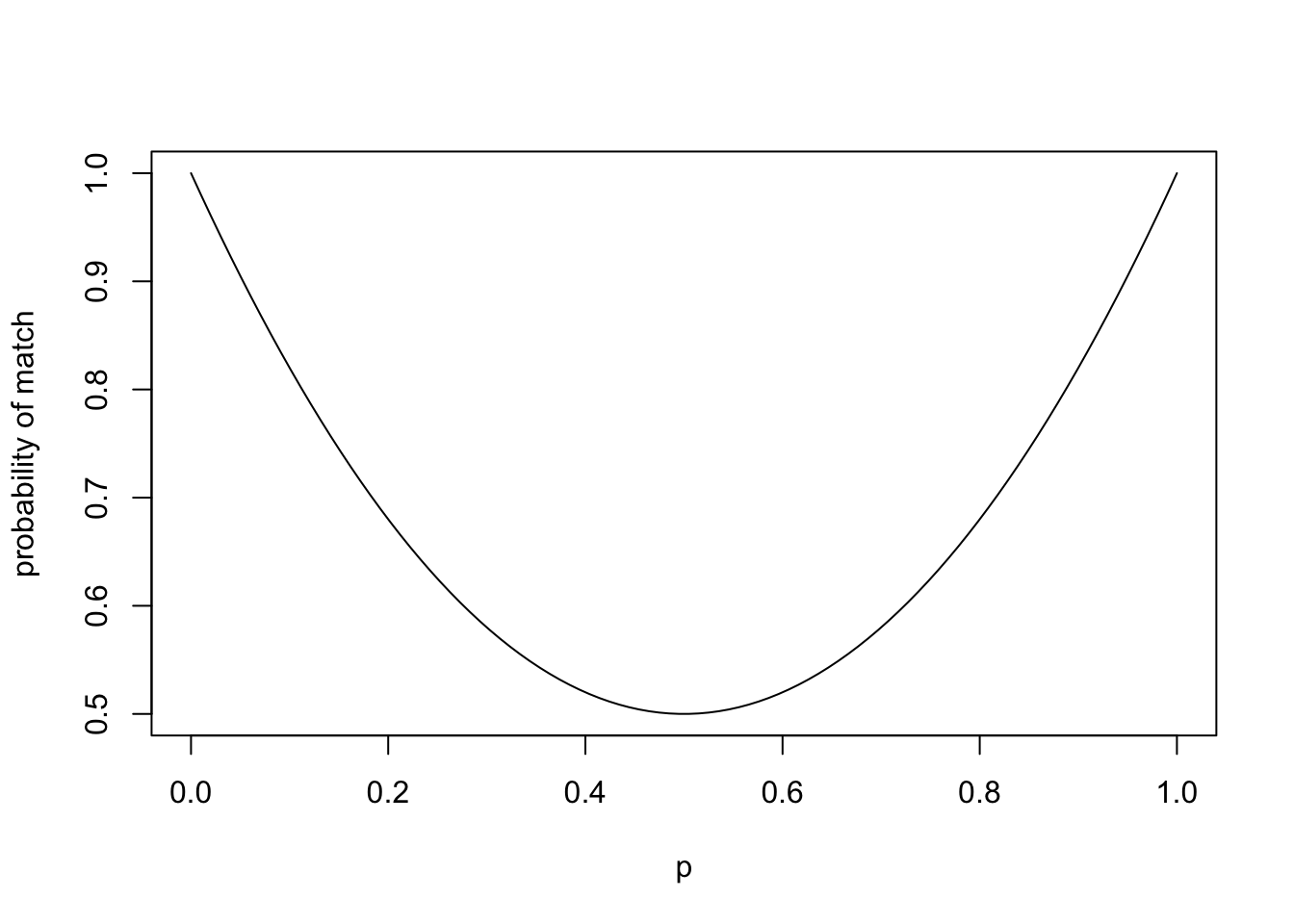

2.29.4 Part (d)

The probability of a match is p^2 + (1-p)^2, so the probability of a non-match is 1 - p^2 - (1-p)^2. If the probability of a convex side up is 0.45, then the probability of a match is:

P(\text{match}) = 0.45^2 + (1-0.45)^2 = 0.505

and the probability of a non-match is:

P(\text{non-match}) = 1 - 0.505 = 0.495

2.29.5 Part (e)

Since the probability of match is slightly higher than the probability of non-match, the captains should call “same” (assuming that they want to play offence first) but the difference is small enough that it doesn’t really matter.

2.29.6 Part (f)

The two-frisbee flip is better than a single-frisbee flip for deciding the offense because the probability of match or non-match is almost a fair coin flip, whereas the probability of a single frisbee is more bias towards the concav side.

2.30 Problem 2.30

Suppose there is a new test that detects whether people have a disease. If a person has the disease, then the test correctly identifies that person as being sick 99.9% of the time (sensitivity of the test). If a person does not have the disease, then the test correctly identifies the person as being well 97% of the time (specificity of the test). Suppose that 2% of the population has the disease. Find the probability that a randomly selected person has the disease given that they test positive for the disease.

We can use Bayes’ theorem to solve this problem:

P(H|E) = \frac{P(E|H)P(H)}{P(E)}

P(E) is more conveniently expressed as:

P(E) = P(E|H)P(H) + P(E|\neg H)P(\neg H)

We know that P(H) = 0.02, P(\neg H) = 0.98, P(E|H) = 0.999 and P(E|\neg H) = 0.03 (false positives). Then We can calculate P(H|E) as follows:

P(H|E) = \frac{0.999 \cdot 0.02}{0.999 \cdot 0.02 + 0.03 \cdot 0.98} = 0.40

2.31 Problem 2.31

Suppose that there are two boxes containing marbles. Box 1 contains 3 red and 4 blue marbles. Box 2 contains 2 red and 5 blue marbles. A single die is tossed, and if the result is 1 or 2, then a marble is drawn from box 1. Otherwise, a marble is drawn from box 2.

balls

1. What is the probability that the marble drawn is red?
2. What is the probability that the marble came from box 1 given that the marble is red?

2.31.1 Part (a)

We can define the following events:

• A: the die is 1 or 2
• B: the die is 3, 4, 5 or 6
• C: the marble is red
• D: the marble is blue

We can calculate the probability of the marble using the law of total being red as follows:

P(C) = P(C|A)P(A) + P(C|B)P(B)

We know that P(A)=\frac{2}{6}, P(B)=\frac{4}{6}, P(C|A)=\frac{3}{7} and P(C|B)=\frac{2}{7}. So we can calculate P(C) as follows:

P(C) = \frac{3}{7} \cdot \frac{2}{6} + \frac{2}{7} \cdot \frac{4}{6} = \frac{11}{42} = 0.26

2.31.2 Part (b)

We can use Bayes’ theorem to calculate the probability that the marble came from box 1 given that the marble is red:

P(A|C) = \frac{P(C|A)P(A)}{P(C)}

Using the values from part (a), we can calculate P(A|C) as follows:

P(A|C) = \frac{\frac{3}{7} \cdot \frac{2}{6}}{\frac{11}{42}} = \frac{6}{11} = 0.54

2.32 Problem 2.32

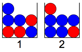
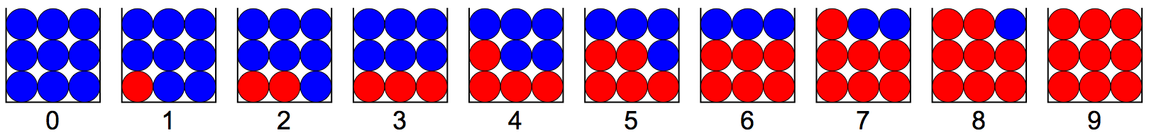
Suppose that you have 10 boxes, numbered 0-9. Box i contains i marbles, and 9-i blue marbles.

balls

You perform the following experiment. Pick a box at random, draw a marble and record its color. Replace the marble back in the box, and draw another marble from the same box and record its color. Replace the marble back in the box, and draw another marble from the same box and record its color. So, all three marbles are drawn from the same box.

1. If you draw three consecutive red marbles, what is the probability that a fourth marble drawn from the same box will also be red?
2. If you draw three consecutive red marbles, what is the probability that you chose box 9?

2.32.1 Part (a)

Let’s first calculate the probability of drawing three consecutive red marbles from a box. We will use conditional probability to solve this problem. Let’s denote the event of drawing three consecutive red marbles as R_{3}, and the event of choosing a box i as B_{i}.

The probability of drawing three consecutive red marbles can be expressed as follows:

P(R_{3}) = \sum_{i=0}^{9} P(R_{3}|B_{i})P(B_{i})

Since we have 10 boxes (numbered 0-9) and we select a box at random, the probability of choosing any box i is:

P(B_{i}) = \frac{1}{10}

Now, let’s calculate the probability of drawing three consecutive red marbles given that we have chosen box i represented by P(R_{3} | B_{i}). The probability of drawing a red marble on box i is \frac{i}{9}. Since we replace the marble after drawing, the probability remains the same for each draw. Therefore, the probability of drawing three consecutive red marbles from box i is:

P(R_{3} | B_{i}) = \left(\frac{i}{9}\right)^{3}

Now, we can calculate the probability of drawing three consecutive red marbles (we can trivially discard i=0):

P(R_{3}) = \frac{1}{10} \cdot \sum_{i=1}^{9} \left(\frac{i}{9}\right)^{3} = 0.277

Now, we want to calculate the probability that the fourth marble drawn from the same box will also be red, given that we have drawn three consecutive red marbles. Let’s denote this event as R_{4} (for the fourth red marble). We need to compute P(R_{4} | R_{3}).

We can apply Bayes’ theorem:

P(R_{4} | R_{3}) = \frac{P(R_{3} | R_{4}) \cdot P(R_{4})}{P(R_{3})}

We know that P(R_{3}) = 0.277, and P(R_{3} | R_{4}) = 1 (because the probability of getting 3 red marbles consecutive given that we have 4 red marbles consecutive is 1). Therefore, the only missing part is P(R_{4}) wich can be calculated as follows:

P(R_{4}) = \sum_{i=1}^{9} P(R_{4} | B_{i})P(B_{i})

P(R_{4}) = \frac{1}{10} \cdot \sum_{i=1}^{9} \left(\frac{i}{9}\right)^4 = 0.233

finally, we can calculate P(R_{4} | R_{3}):

P(R_{4} | R_{3}) = \frac{1 \cdot 0.233}{0.277} = 0.84

We can simulate this experiment as follow:

event_a_and_b <- replicate(100000, {
    box <- sample(x = 0:9, size =1)
    marbles <- sample(c(rep("red", box), rep("blue", 9 - box)), 4, replace = TRUE)
    all(marbles == "red")
})

event_b <- replicate(100000, {
    box <- sample(x = 0:9, size =1)
    marbles <- sample(c(rep("red", box), rep("blue", 9 - box)), 3, replace = TRUE)
    all(marbles == "red")
})

mean(event_a_and_b) / mean(event_b)

[1] 0.8350382

2.32.2 Part (b)

Let’s denote the event of choosing box 9 as B_{9}. We want to calculate P(B_{9} | R_{3}). We can apply Bayes’ theorem:

P(B_{9} | R_{3}) = \frac{P(R_{3} | B_{9}) \cdot P(B_{9})}{P(R_{3})}

The probability of getting three consecutive red marbles given that we have chosen box 9 is P(R_{3} | B_{9}) = \left(\frac{9}{9}\right)^3 = 1. The probability of choosing box 9 is P(B_{9}) = \frac{1}{10}. The probability of getting three consecutive red marbles is P(R_{3}) = 0.277. Therefore, we can calculate P(B_{9} | R_{3}) as follows:

P(B_{9} | R_{3}) = \frac{1 \cdot \frac{1}{10}}{0.277} = 0.36

We can simulate this experiment as follow:

event_a_and_b <- replicate(100000, {
    box <- sample(x = 0:9, size =1)
    marbles <- sample(c(rep("red", box), rep("blue", 9 - box)), 3, replace = TRUE)
    all(marbles == "red") && box == 9
})

event_b <- replicate(100000, {
    box <- sample(x = 0:9, size =1)
    marbles <- sample(c(rep("red", box), rep("blue", 9 - box)), 3, replace = TRUE)
    all(marbles == "red")
})

mean(event_a_and_b) / mean(event_b)

[1] 0.363971

2.33 Problem 2.33

How many ways are there of getting 4 heads when tossing 10 coins?

using the binomial coefficient:

{10 \choose 4} = \frac{10!}{4! \cdot 6!} = 210

2.34 Problem 2.34

How many ways are there of getting 4 heads when tossing 10 coins, assuming that the 4th head came on the 10th toss?

If we know that the 4th head came on the 10th toss, then we must have gotten exactly 3 heads in the first 9 tosses. We can count the number of ways to get 3 heads in 9 tosses using the binomial coefficient:

{9 \choose 3} = \frac{9!}{3! \cdot 6!} = 84

2.35 Problem 2.35

Six standard six-sided dice are rolled.

1. How many outcomes are there?
2. How many outcomes are there such that all of the dice are different numbers?
3. What is the probability that you obtain six different numbers when you roll six dice?

2.35.1 Part (a)

The number of outcomes is 6^{6} = 46656

2.35.2 Part (b)

The first die can be any of the six numbers. The second die must be one of the remaining five numbers (since we can’t repeat the number from the first die), the third die must be one of the remaining four numbers, and so on. Therefore, the number of outcomes in which all six dice are different is:

The number of outcomes is 6 \cdot 5 \cdot 4 \cdot 3 \cdot 2 \cdot 1 = 720

2.35.3 Part (c)

The probability of getting six different numbers when rolling six dice is:

P(E) = \frac{720}{46656} = 0.0154

2.36 Problem 2.36

A box contains 5 red marbles and 5 blue marbles. Six marbles are drawn without replacement.

1. How many ways are there of drawing the 6 marbles? Assume that getting all 5 red marbles and the first blue marble is different than getting all 5 red marbles and the second blue marble, for example.
2. How many ways are there of drawing 4 red marbles and 2 blue marbles?
3. What is the probability of drawing 4 red marbles and 2 blue marbles?

2.36.1 Part (a)

The number of ways of drawing 6 marbles is:

{6 \choose 10} = \frac{10!}{6! \cdot 4!} = 210

2.36.2 Part (b)

The number of ways of drawing 4 red marbles and 2 blue marbles is:

{5 \choose 4} \cdot {5 \choose 2} = \frac{5!}{4! \cdot 1!} \cdot \frac{5!}{2! \cdot 3!} = 50

2.36.3 Part (c)

The probability of drawing 4 red marbles and 2 blue marbles is:

P(E) = \frac{50}{210} = 0.238

We can simulate this experiment as follow:

event <- replicate(100000, {
    marbles <- sample(c(rep("red", 5), rep("blue", 5)), 6, replace = FALSE)
    sum(marbles == "red") == 4 && sum(marbles == "blue") == 2
})

mean(event)

[1] 0.23855